This is the fifth post (#5) in the Efficient ML series. If Low-bit Quantization #4 was about recipes for quantizing a finished model well after the fact (PTQ), this time we push quantization into the training loop itself: QAT. The code lives in
qat.ipynbat github.com/warpspaceinc/efficient-ml-practice, and every plot and table below is our own number, measured by actually running that code.
Where PTQ breaks down
Every quantization we have done so far was PTQ (Post-Training Quantization): taking a trained FP32 model and moving it onto an integer grid after the fact. It works well for big models. With INT8 PTQ, ResNet-50 loses −0.1% and GoogleNet is essentially lossless.
The problem is small models. With the very same INT8 PTQ, the numbers are striking1. For example:
| Model | FP32 | INT8 PTQ (per-tensor) |
|---|---|---|
| ResNet-50 | 76.1% | −0.1% |
| MobileNetV1 | 70.9% | 0.1% |
| MobileNetV2 | 71.9% | 0.1% |
MobileNet goes from 70.9% down to 0.1%: it dies completely. The more compact a model is (built to save every parameter), the less redundancy it has, and so nowhere to absorb quantization error. And this shows up as you drop bits (below 4-bit) regardless of model size.
Our own MNIST MLP (784→256→128→10) reproduces exactly the same thing. PTQ-ing the weights at each bit-width:
- 8-bit: 97.1% (fine)
- 4-bit: 96.9%
- 3-bit: 94.9%
- 2-bit: 13.6%, essentially collapsed to near-random (10%)
So what do we do? The answer is as simple as it is powerful. “If we’re going to run inference quantized anyway, let’s train quantized from the start.”
QAT: mimicking quantization during training
The heart of QAT (Quantization-Aware Training) is fake quantization. Into the training forward pass, we pre-simulate the quantization that will happen at inference. The scheme boils down to three principles2.
- Keep the FP32 master weight $W$ around. The thing being learned is this continuous value.
- In the forward pass only, quantize-and-restore (fake-quant) weights and activations, so the ops run on values sitting on the integer grid.
- At inference, use only these quantized weights.
As a formula, it is simply inserting the affine mapping from #2 into the forward pass, for weights and for outputs (activations):
$$Q(W) = S_W\, q_W, \qquad Q(Y) = S_Y\,(q_Y - Z_Y)$$where $q_W = \mathrm{round}(W/S_W)$ snaps to the grid with round, then multiplies the scale back to return to a real number (hence “fake”: the value sits on the grid, but the op itself runs in FP32). Since training now proceeds on this grid, the model tunes itself so that “the output stays good even when this weight is crushed to 2 bits.” Instead of enduring quantization error after the fact, we bake it into the training objective from the start.
But this creates one decisive problem.
STE: round has zero derivative, so how does it learn?
The heart of fake quantization is the round function. And round is a staircase: its slope is 0 almost everywhere, and infinite only at the grid boundaries.
Follow the backprop chain rule literally and it is a disaster.
$$g_W = \frac{\partial L}{\partial W} = \frac{\partial L}{\partial Q(W)} \cdot \frac{\partial Q(W)}{\partial W} = \frac{\partial L}{\partial Q(W)} \cdot 0 = 0$$Every weight’s gradient becomes 0. Training can’t take a single step. A single round blocks the entire backward pass.
The fix is the STE (Straight-Through Estimator)34. The idea is brazenly simple. “Use round in the forward pass, but in the backward pass pretend it wasn’t there and let the gradient pass straight through.” That is, when differentiating the quantizer, treat it as the identity.
$$g_W = \frac{\partial L}{\partial W} \;\approx\; \frac{\partial L}{\partial Q(W)}$$Staircase forward, slope-1 backward. This “lie” is what makes QAT work.
The fun part is where this brazen trick comes from. STE was introduced in passing by the godfather of deep learning, Geoffrey Hinton, in a 2012 Coursera lecture3, and formalized the next year by Bengio et al.4. That same Hinton went on from the Turing Award (2018) to a 2024 Nobel Prize in Physics, and remains vigorously active in AI discourse to this day. A one-liner tossed off in a lecture over a decade ago still underpins low-bit training today.
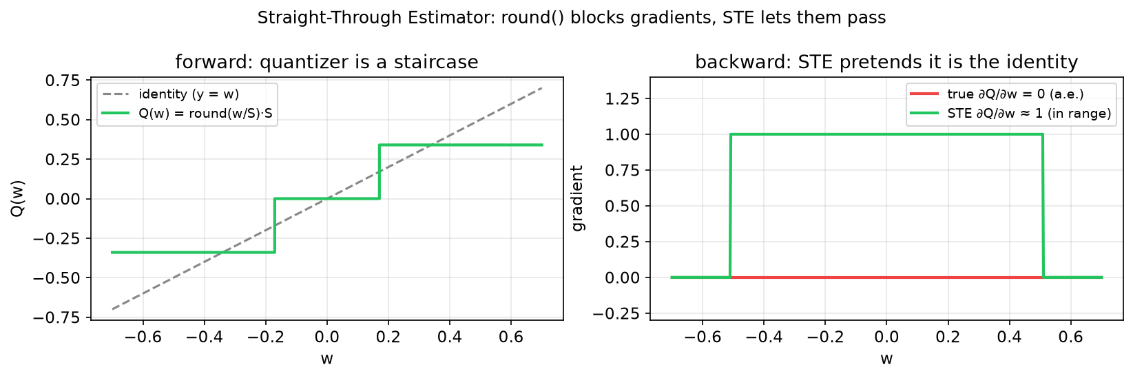
The left is the forward. $Q(w)$ approximates the dashed identity ($y=w$) as a staircase. The right is the backward. The true derivative is 0 (red), but the STE passes the gradient through as 1 (green) inside the representable range. Outside the range (the clipped region) it is left at 0, so values off the grid get no signal.
Play with it directly below. It is a computation graph with a single scalar weight $w$ ($w \to Q(w) \to \hat y=Q(w)\cdot x \to L=\tfrac12(\hat y-t)^2$). Move the sliders for weight $w$, input $x$, and target $t$, and the loss and gradients update in real time: watch especially how, in the backward pass, the true derivative (0) and the STE gradient diverge.
In PyTorch it takes a single custom autograd.Function: quantize in forward, pass-through (plus a clip mask) in backward.
class FakeQuantSTE(torch.autograd.Function):
    @staticmethod
    def forward(ctx, w, n_bits):
        qmax = 2 ** (n_bits - 1) - 1
        S = w.detach().abs().max() / qmax + 1e-12       # per-tensor symmetric scale
        q = torch.clamp(torch.round(w / S), -qmax, qmax)  # snap to grid
        ctx.save_for_backward((w.abs() <= S * qmax).to(w.dtype))  # clip mask
        return q * S                                     # dequantize (fake-quant)
    @staticmethod
    def backward(ctx, g):
        (mask,) = ctx.saved_tensors
        return g * mask, None          # STE: pass inside range, 0 outside
And QAT training is just the ordinary loop with this fq wrapped around the weights in the forward pass. The master weight stays FP32, and thanks to the STE the gradient flows back to that master.
def qat_forward(x):
    x = F.relu(F.linear(x, fq(fc1.weight, b), fc1.bias))
    x = F.relu(F.linear(x, fq(fc2.weight, b), fc2.bias))
    return F.linear(x, fq(fc3.weight, b), fc3.bias)
Measured directly: PTQ vs QAT
On the same MNIST MLP, at the same bit-widths, we measured PTQ (quantize after training) and QAT (fine-tune the FP32 model for 2 epochs with fake-quant) side by side.
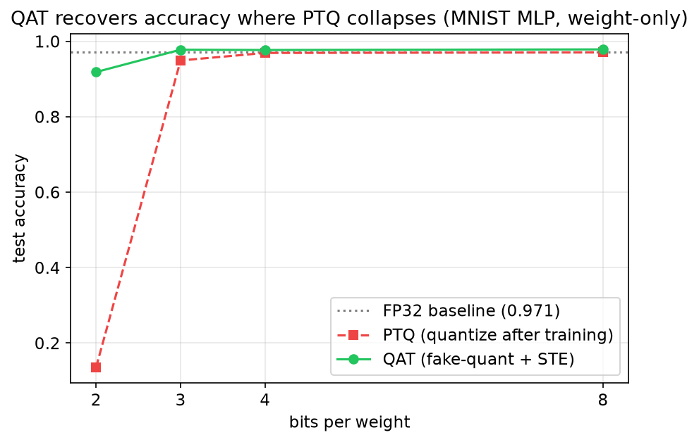
| bits | PTQ | QAT | FP32 |
|---|---|---|---|
| 8 | 97.1% | 97.9% | 97.1% |
| 4 | 96.9% | 97.7% | 97.1% |
| 3 | 94.9% | 97.8% | 97.1% |
| 2 | 13.6% | 91.9% | 97.1% |
The picture to read is clear.
- At 8-bit, both are lossless. Where there’s headroom, you don’t need QAT.
- The gap explodes as bits drop. At 2-bit PTQ dies at 13.6% (random-level), while QAT rescues it up to 91.9%. It is the exact same pattern as MobileNetV1 (INT8 PTQ 0.1%, QAT ~70%)1.
- QAT sometimes edges past the baseline (3/4-bit): the effect of a few extra epochs of fine-tuning.
The crux is this. PTQ was the problem of “fitting already-fixed weights onto the grid as well as possible.” QAT is the problem of “finding the best weights on the grid from the start.” The degrees of freedom differ, and so the results diverge at low bits.
Run it yourself
The plots and tables above come straight from running the notebook below. Runtime → Run all and you’re done.
- 📓
qat.ipynb: fake quantization, STE (autograd.Function), PTQ vs QAT comparison
After STE: learning the scale and clip too, LSQ · PACT
So far our fake-quant set the scale $S$ by a fixed heuristic, $|W|_{\max}/q_{\max}$. STE only routes the weight gradient; the grid spacing $S$ itself was never learned. The next improvement is to learn that scale and clip too.
LSQ: learning the step size. LSQ (Learned Step Size Quantization)5 makes $S$ a learnable parameter. In $Q(w)=\mathrm{round}(\mathrm{clip}(w/S))\cdot S$ it computes $\partial Q/\partial S$ sensitively to quantization state transitions and optimizes it by gradient: inside the range $\partial Q/\partial S = \mathrm{round}(w/S) - w/S$ (the gap between the grid value and the continuous value), outside the range $\pm q_{\max}$. The effect is large at low bits. Comparing our MLP against fixed-scale QAT:
| bits | QAT (fixed scale) | QAT + LSQ (learned scale) |
|---|---|---|
| 4 | 97.9% | 97.7% |
| 3 | 97.6% | 97.9% |
| 2 | 92.3% | 96.7% |
At 2-bit, 92% rises to 97%. Just by letting the data decide one grid spacing, the last gap is filled. The tighter the low-bit budget, the more “what to set the scale to” decides accuracy.
PACT: learning the activation clip range. Weights have a fixed min/max once training ends, but activations (ReLU outputs) have an open-ended range. Where #4 chose the clip point with KL, PACT6 makes that clip threshold $\alpha$ a learnable parameter. It replaces ReLU with $\mathrm{clip}(x, 0, \alpha)$ and learns $\alpha$ by gradient, letting the data set the range of activation quantization. Just as LSQ learns the weight’s scale, PACT learns the activation’s clip.
And as we enter the LLM era, this story goes much further: all the way to BitNet, which trains from scratch in ternary {−1, 0, +1}, and the move toward pretraining in FP4. That we’ll cover separately in a dedicated LLM-quantization post.
Wrap-up
- PTQ works for big models but breaks on small models and low bits. MobileNet INT8 dies at 0.1%, and our MLP collapses to 13.6% at 2-bit PTQ.
- QAT inserts fake quantization into the training forward pass, letting the model tune itself to be good in the quantized state. The FP32 master weight is preserved.
- round’s gradient is 0, so naively nothing learns, but the STE treats quantization as the identity in the backward pass and lets the gradient through.
- Result: at 2-bit, PTQ 13.6% rises to QAT 91.9%. The lower the bits, the more QAT is worth.
That wraps up the quantization arc (#2 · #4 · #5). From data types to quantization, pruning, low-bit, and QAT, we’ve walked the tools for making models small and fast, from concept to measurement.
References
Krishnamoorthi. Quantizing Deep Convolutional Networks for Efficient Inference: A Whitepaper. arXiv 2018. (original source of the MobileNet PTQ/QAT numbers) ↩︎ ↩︎
Jacob et al. Quantization and Training of Neural Networks for Efficient Integer-Arithmetic-Only Inference. CVPR 2018. ↩︎
Hinton et al. Neural Networks for Machine Learning. Coursera Lecture, 2012. (origin of the STE) ↩︎ ↩︎
Bengio et al. Estimating or Propagating Gradients Through Stochastic Neurons for Conditional Computation. arXiv 2013. ↩︎ ↩︎
Esser et al. Learned Step Size Quantization. ICLR 2020. ↩︎
Choi et al. PACT: Parameterized Clipping Activation for Quantized Neural Networks. arXiv 2018. ↩︎