Efficient ML #4, Low-bit Quantization: Fighting Outliers

This is the fourth post (#4) in the Efficient ML series. In Quantization #2 we saw that “8 bits is free, 2 bits collapses”; this time we look at why it collapses, and how to bring it back. The code lives in low-bit-quantization.ipynb at github.com/warpspaceinc/efficient-ml-practice, and every plot and table below is our own number, measured by actually running that code.

FP4, an absurd bet

There is a line in NVIDIA Blackwell’s spec sheet that makes you look twice: the FP4 tensor core delivers exactly 2× the throughput of FP8. Halving the bits doubles the throughput: simple arithmetic. The problem is the FP4 (E2M1) format itself. One sign bit + 2 exponent bits + 1 mantissa bit. That makes exactly 15 representable values:

$$\pm\{0.5,\ 1,\ 1.5,\ 2,\ 3,\ 4,\ 6\}\ \cup\ \{0\}$$

Unlike INT4’s uniform grid, FP4 is dense near zero (spacing 0.5 near the center, 2.0 at the edge). Given that weights cluster in a bell shape around zero, that’s a sensible layout. But 15 values are still 15 values.

The representable range also matters: it is just [−6, 6]. To squeeze real-valued weights into that narrow window, you have to divide them by a scale factor $S$. And how you choose that scale decides whether low-bit quantization lives or dies. The rest of this post is that story.

We experiment with the same MNIST MLP as #2 (784→256→128→10, FP32 accuracy 97.4%).

---

1. The culprit: one outlier erases a layer

The simplest scale design uses a single scale for the whole tensor, called per-tensor: pick $S$ so that the largest-magnitude weight lands on FP4’s maximum of 6, i.e. $S = |W|_{\max} / 6$. Nothing gets clipped, so it looks safe.

But look at that formula again and there is something alarming in it: a single maximum value determines the spacing of the entire grid. If the max grows, the scale grows, the grid becomes coarser, and the resolution for the vast majority of weights sitting near zero degrades. So what happens if, for whatever reason, there is even one abnormally large value, an outlier?

Let’s find out. In a copy of fc1’s weights (200K elements), we blow up exactly one element to 50× the max, then measure the damage to the remaining weights after FP4 quantization.

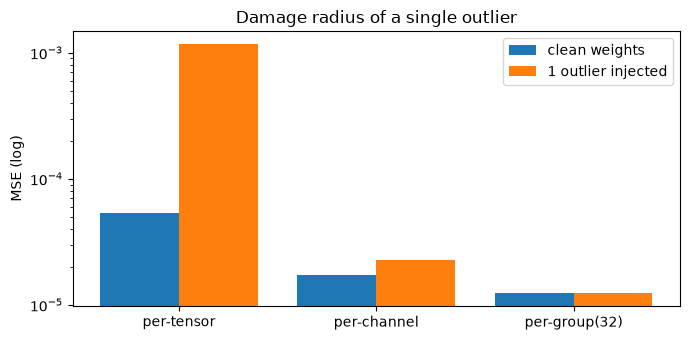
scale granularity	MSE (clean)	MSE (with outlier)	increase
per-tensor	5.4e-05	1.2e-03	22×
per-channel	1.7e-05	2.3e-05	1×
per-group(32)	1.2e-05	1.2e-05	1×

The per-tensor “22×” is worse than the number suggests. Follow the chain: the outlier drags $|W|_{\max}$ up 50×, so the scale grows 50×. The smallest non-zero FP4 level ($0.5 \times S$) then becomes larger than every normal weight ($|w| \le 0.3$). From every normal weight’s point of view, the nearest grid point is now zero. In other words, nearly all 200K weights snap to zero. One outlier has erased the whole layer.

This is not just an artificial scenario. The real-world case shown in the MIT 6.5940 lecture¹ is MobileNetV2, whose first depthwise layer has per-channel weight ranges differing by more than 100×. Most low-bit quantization failures follow this pattern: one outlier poisons the scale and kills the resolution of everything else.

2. Cure ①: chop the scale into pieces, group quantization

The table above already shows the cure. If the essence of the problem is “one outlier poisons the scale of the entire tensor,” then shrink the territory each scale is responsible for. Reduce the blast radius of the damage.

• per-channel: one scale per channel (row). The outlier’s damage is confined to its own row (784 elements in fc1).
• per-group(32): one scale per 32 elements. The damage is confined to just 31 group-mates. That is why the MSE in the table doesn’t budge even with the outlier injected.

This per-group scheme is exactly the micro-tensor scaling that NVIDIA Blackwell supports in hardware. And its industry-standard form is MXFP4: FP4 elements plus one shared scale per 32 elements. This is why the absurd bet of FP4 works in practice: group scales have shrunk an outlier’s blast radius to 31 elements.

3. The cost of all those scales: 2^k scales and effective bits

Of course, it isn’t free. For fc1, the number of scales grew from 1 (per-tensor) to 6,272 (per-group). Those scales are data too; they must be stored and multiplied. MXFP4 keeps this cost down with two ideas.

First, restrict scales to powers of two. MXFP4 group scales are not FP32 numbers but 8-bit exponents (E8M0), i.e. values of the form $2^k$. Scale multiplication then becomes exponent addition, which is extremely cheap in hardware. The trade-off is that scales can only move in factors of 2, so they can miss the optimum. Measuring that penalty:

layer	group32 + FP scale	group32 + 2^k scale	penalty
fc1	1.23e-05	1.58e-05	1.28×
fc2	2.66e-05	3.62e-05	1.36×
fc3	6.12e-05	6.30e-05	1.03×

An MSE penalty of 1.0–1.4×. Compared with the 22× an outlier causes, that is cheap insurance, a different order of magnitude entirely.

Second, account for the overhead in effective bits. The true storage cost per element is:

$$\text{effective bits} = \text{element bits} + \frac{\text{scale bits}}{\text{group size}}$$

MXFP4 comes to $4 + 8/32 = 4.25$ bits. With FP16 scales it would have been 4.5; the $2^k$ trick means an 8-bit exponent suffices, landing at 4.25. NVIDIA’s VS-Quant² stacks the same idea hierarchically: a cheap INT4 scale per 16 elements, with a single expensive FP scale per tensor correcting the absolute magnitude. It also lands on 4.25 bits.

4. Putting it together as FP4 accuracy

Finally, we quantize all of the MLP’s weights to 4 bits with each scheme and measure MNIST accuracy.

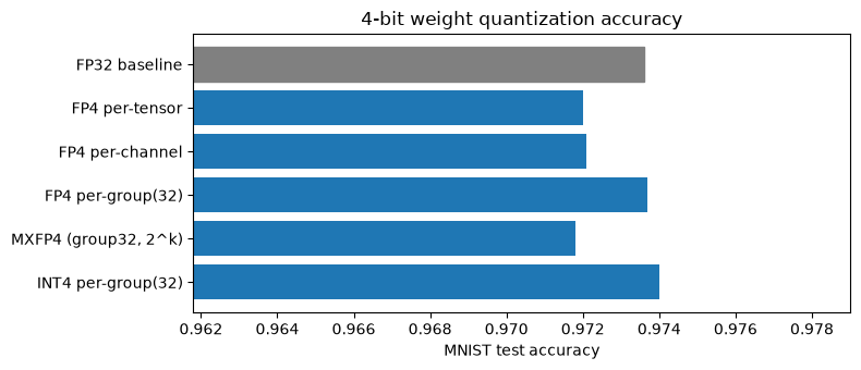
scheme	accuracy	effective bits
FP32 baseline	97.36%	32
FP4 per-tensor	97.20%	4.0
FP4 per-group(32)	97.37%	4.5
MXFP4 (group32, 2^k)	97.18%	4.25

MXFP4 sits within 0.2pp of the baseline at 7.5× compression. This is the moment 4-bit weights stop being an absurd bet and become a practical choice.

---

Three questions that remain

That was the story of packing weights into 4 bits. Group scales (cure ①) shrank the outlier’s blast radius and made 4-bit weights practical. But three questions remain.

1. Everything so far was about weights. What about activations, whose values change with every input?
2. After fixing the scale, is “round each value to the nearest grid point” really the best move?
3. Instead of containing outliers, can we eliminate them altogether?

We answer each with one weapon (cure) used in practice.

5. Cure ②: clip the activations, KL clipping

Weights are fixed once training ends, so their min/max is known exactly. Activations change range with every input. So before deployment, you run a few batches of representative inputs (calibration data) through the model and collect statistics about each layer’s activation range.

The question is which statistic to base the scale on. The observed maximum? Then the same disease from the weight story returns, because ReLU outputs have very long tails. In our measurements, fc1’s activation max is 19.7, while 99.9% of the values sit below 9.7. Scaling by the max means sacrificing the resolution of 99.9% of values for the top 0.1%.

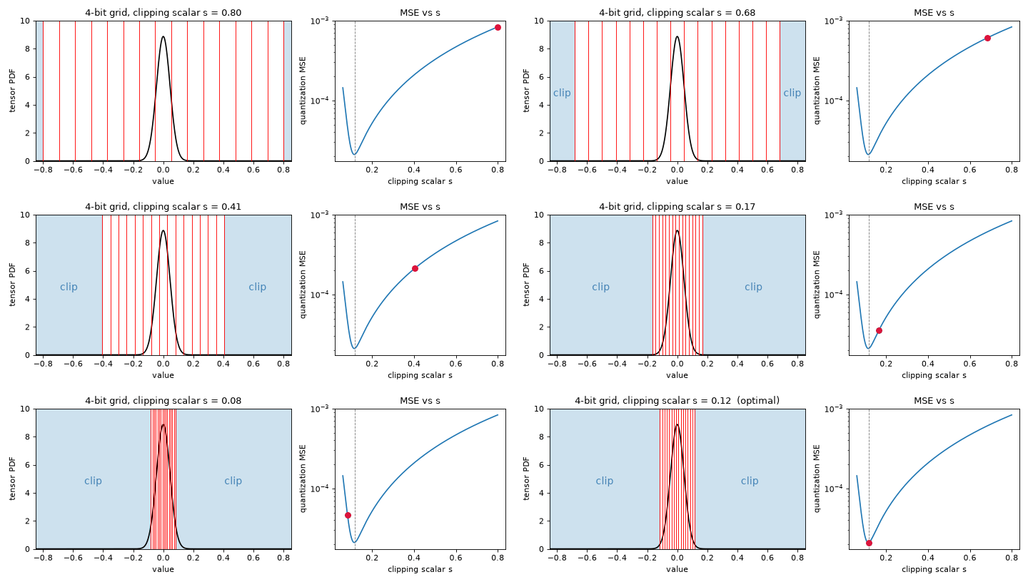
So clipping somewhere should pay off. But where? Clip too early and the clipped values lose their information (saturation loss); clip too late and the grid becomes coarse (rounding loss). The optimum lies somewhere between.

The animation below shows that trade-off. Tighten a 4-bit grid (16 red lines) over a bell-shaped distribution, starting from the max: at first the grid gets denser and the MSE falls steeply, but the moment it starts cutting into the distribution’s body, saturation loss takes over and the MSE climbs again.

The same U-shape appears in real, large models. The figure below is from NVIDIA’s OCTAV paper³, which measured quantization MSE while sweeping the clipping point on weight and activation layers of ResNet-50. Here MSE is measured element-wise on the tensor, $\mathbb{E}[(Q(x)-x)^2]$, the mean squared difference between each value before and after quantization (not a difference in model outputs). Every layer and bit width shows the U-curve and its optimum (circled), and the lower the bit width, the further inward the optimal clip moves. OCTAV finds this optimum with Newton-Raphson iterations at every training step.

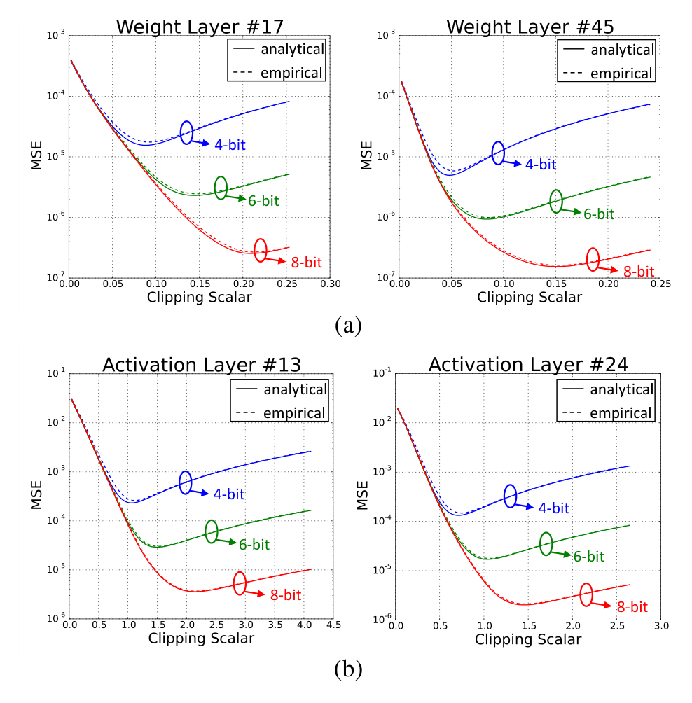
Figure credit: Sakr et al., ICML 2022³, Figure 1.

TensorRT’s solution⁴ treats this as an information-loss minimization problem. For each candidate point T, build P, the original distribution clipped at T, and Q, the same distribution quantized to n levels and then expanded back onto P’s bins (two distributions at different resolutions cannot be compared directly), then compute the KL divergence $D_{KL}(P\|Q)$ between them. The T that minimizes it is the cut that loses the least information. Since the two losses move in opposite directions, the KL curve is U-shaped.

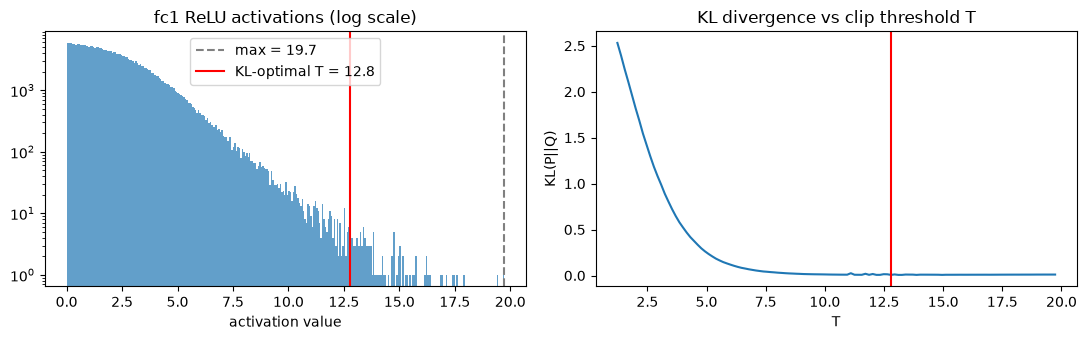
On our MLP, KL picks T = 12.8 (max 19.7). Quantizing activations with it and comparing against the max-based scale:

bits	clip = max	clip = KL
4	97.19%	97.24%
3	96.91%	96.93%
2	91.21%	96.15%

The lower the bit width, the wider the gap. At 2 bits, giving up a few outliers buys back 5 percentage points. The method’s practical strength is that it assumes nothing about the distribution’s shape: whether a layer’s activations decay monotonically or form a bell, it works the same way.

6. Cure ③: learn the rounding, AdaRound

Even with scale and clip decided, one degree of freedom remains: the rounding that sends each value to a grid point. “Round to nearest” (RTN) feels so obvious that it hardly seems like a choice at all, but Qualcomm’s AdaRound⁵ showed it is not optimal.

Here is why. Weights in the same layer multiply the same input and sum into one output. Their individual rounding errors are therefore not independent; they cancel or compound downstream. RTN decides each weight’s rounding by looking only at that weight’s own error, ignoring the interaction entirely. The sum of individual optima is not the collective optimum.

So AdaRound changes the objective. Instead of reconstructing the weights, find the up/down combination that best reconstructs the layer’s output:

$$\arg\min_{\mathbf{V}} \|\mathbf{W}\mathbf{x} - \lfloor\lfloor\mathbf{W}\rfloor + h(\mathbf{V})\rceil\,\mathbf{x}\|_F^2 + \lambda f_{reg}(\mathbf{V})$$

The formula looks busy, but the structure is simple. Each weight’s choice between rounding down ($\lfloor w \rfloor$) and up ($\lfloor w \rfloor + 1$) is relaxed into a continuous value $h(V) \in (0,1)$ and learned by gradient descent, while the regularizer $f_{reg}$ pushes it to 0 or 1 as training ends. No labels, no full retraining; a few calibration batches and a short per-layer optimization suffice. Our notebook runs 800 steps per layer, tens of seconds on CPU.

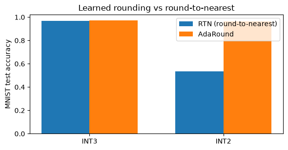
bits	RTN	AdaRound	roundings flipped
INT3	96.83%	97.23%	11.8%
INT2	53.37%	96.56%	12.0%

INT2 is dramatic. Flipping just 12% of the rounding decisions brings accuracy from 53% back to 97%. It shows how expensive the “nearest value” intuition really was at low bit widths.

7. Cure ④: rotate the coordinate system to remove outliers, Hadamard rotation

Every remedy so far coexisted with outliers. We contained them (group scales), cut them off (clipping), or worked around them (AdaRound). The latest LLM quantization methods (QuaRot⁶, SpinQuant⁷) think differently: rotate into a coordinate system where the outliers don’t exist.

What makes this possible is computational invariance. Pick any orthogonal matrix $R$ ($RR^\top = I$), and

$$\mathbf{y} = \mathbf{W}\mathbf{x} = (\mathbf{W}R^\top)(R\,\mathbf{x})$$

Pre-transform the weights to $WR^\top$ and the input to $Rx$, and the output is mathematically identical. The function the model computes stays the same; only the “shape” of the tensors that quantization sees has changed.

Now choose $R$ to be a Hadamard matrix (an orthogonal matrix of ±1 entries divided by $\sqrt{n}$) and something magical happens. After rotation, each component becomes a ±average of all the original components. An outlier concentrated in one spot gets smeared across every dimension at $1/\sqrt{n}$ magnitude. The spiky distribution returns to a bell shape.

Try it in the widget below. Rotate a vector concentrated in one axis (like [1, 0]) with the slider, and at 45° the two coordinates become equal, [0.707, 0.707], the length is unchanged while the outlier is split evenly across both axes.

We recreated the outlier scenario from earlier (one weight blown up 50×) on fc2 and rotated it:

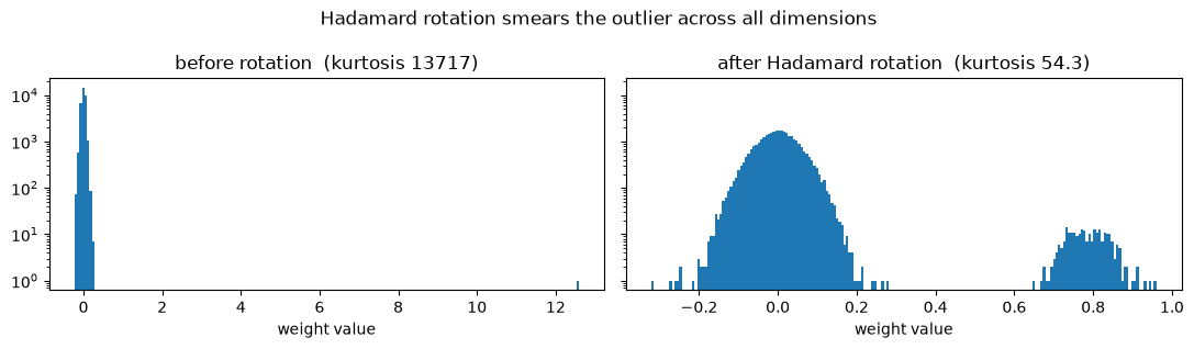
Measured by kurtosis (an indicator of how “normal” a distribution is; a Gaussian scores 3), the weights go from 13,717 to 54, and with both input and output sides rotated (the QuaRot recipe) down to 3.4. The outlier’s statistical trace is gone. Confirming with output error after FP4 quantization:

	per-tensor	per-group(32)
no outlier (reference)	0.059	0.045
outlier, no rotation	0.859	0.043
outlier + Hadamard, input side only	0.197	0.089
outlier + Hadamard, both sides (QuaRot)	0.093	0.067

How to read it: with an outlier, per-tensor is wiped out (0.86), and two-sided rotation revives it to near the reference (0.09). Conversely, per-group gains nothing from rotation, because the group scales were already containing the outlier. This reveals rotation’s character: its benefit grows as scales get coarser. That is why rotation shines exactly where fine-grained scales are hard to attach, most notably the activations in W4A4 pipelines.

The cost profile is attractive too. Group scales carry a storage overhead (+0.25 bits), but rotation adds zero extra storage: $WR^\top$ is precomputed before deployment, and the $Rx$ during inference runs in $O(n \log n)$ thanks to the Hadamard transform’s structure.

One caveat: our experiment is 256-dimensional, so the outlier only shrank by 1/16. Real LLMs have hidden dimensions of 4096 or more, shrinking it by 1/64 or better. The bigger the model, the more complete the rotation trick becomes. This is what made W4A4 inference on LLaMA-2 70B work in QuaRot, and SpinQuant goes one step further by learning the rotation matrices themselves.

---

Run it yourself

The plots and tables above come from running the notebook below. Runtime then Run all is all it takes.

• 📓 low-bit-quantization.ipynb: FP4/MXFP4 group quantization, outlier experiments, KL clipping, AdaRound, Hadamard rotation

Takeaways: four cures in one table

Low-bit quantization is a war against the worst value (the outlier), not the average one, because the scale is always chained to the maximum. Gathering the four cures of that war into one table:

cure	idea	cost	our measurement
① Group scales (MXFP4)	confine damage to 31 group-mates	+0.25 bit	−0.2pp from baseline at FP4
② KL clipping	sacrifice a few outliers, keep resolution	calibration search	+5pp at 2-bit
③ AdaRound	learn rounding against layer outputs	short per-layer optimization	53→97% at INT2
④ Hadamard rotation	rotate into an outlier-free basis	zero extra storage	9× lower per-tensor error

• The four cures aren’t competitors but orthogonal tools. Real W4A4 pipelines combine rotation (outlier removal) + group scales (absorbing residual variance) + clipping (activations).

References

Song Han. MIT 6.5940 TinyML and Efficient Deep Learning Computing, Lecture 6: Quantization Part II. efficientml.ai ↩︎
Dai et al. VS-Quant: Per-Vector Scaled Quantization for Accurate Low-Precision Neural Network Inference. MLSys 2021. ↩︎
Sakr et al. Optimal Clipping and Magnitude-aware Differentiation for Improved Quantization-aware Training. ICML 2022. ↩︎ ↩︎
Szymon Migacz. 8-bit Inference with TensorRT. GTC 2017. ↩︎
Nagel et al. Up or Down? Adaptive Rounding for Post-Training Quantization. PMLR 2020. ↩︎
Ashkboos et al. QuaRot: Outlier-Free 4-Bit Inference in Rotated LLMs. NeurIPS 2024. ↩︎
Liu et al. SpinQuant: LLM Quantization with Learned Rotations. 2024. ↩︎